[Solved] Conditional Formatting Based on Another Cell: the Solution

Conditional formatting is a powerful feature in spreadsheet applications like Excel and Google Sheets that allows you to apply formatting rules to cells based on their values or the values of other cells. One of the most useful applications of conditional formatting is the ability to format a cell based on the value of another cell. This can be particularly helpful when you need to highlight or emphasize specific data points based on certain conditions or criteria.

In this article, we'll explore how to use conditional formatting based on another cell in both Excel and Google Sheets, providing step-by-step instructions and detailed examples to help you master this technique.

Conditional Formatting Based on Another Cell: What Does It Mean?

Before we dive into the specifics, let's first understand what it means to apply conditional formatting based on another cell. Essentially, this technique allows you to set formatting rules for a cell (or range of cells) based on the value or condition of a different cell (or range of cells).

For example, you might want to highlight a cell in green if the value in another cell meets a certain condition, such as being greater than a specific number or containing a particular text string. This can be incredibly useful for visualizing data relationships, identifying outliers, or drawing attention to important information.

Google Sheets AI Formula Generator | Formula Builder | Anakin.ai

Want to effortlessly create Google Sheets Formulas? This AI tool is here to help you easily create Google Sheets Formula Generator with ease!

Sam AltwomanSam Altwoman2

Conditional Formatting Based on Another Cell in Excel

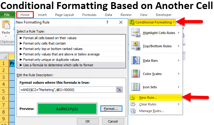
In Excel, you can apply conditional formatting based on another cell by using the "Conditional Formatting" feature and specifying the appropriate rules and conditions. Here's a step-by-step guide:

1. Select the cell or range of cells you want to format based on another cell.
2. Go to the "Home" tab and click on "Conditional Formatting."
3. In the "Conditional Formatting" dropdown menu, select "New Rule."
4. In the "New Formatting Rule" dialog box, select the desired rule type (e.g., "Format only cells that contain," "Format only top or bottom ranked values," etc.).
5. Depending on the rule type you selected, you'll need to specify the condition or criteria. For example, if you choose "Format only cells that contain," you can enter a formula that references the cell you want to base the formatting on.
6. Click on the "Format" button to choose the desired formatting style (e.g., cell color, font style, etc.).
7. Click "OK" to apply the conditional formatting rule.

How to Highlight Cells Based on Another Cell's Value in Excel

Let's say you have a spreadsheet with sales data, and you want to highlight the cells in column C (Total Sales) based on the corresponding values in column B (Target Sales). Specifically, you want to highlight the cells in green if the Total Sales value is greater than or equal to the Target Sales value, and in red if it's less than the Target Sales value.

Here are the steps:

1. Select the range of cells in column C that you want to format (e.g., C2:C100).
2. Go to "Home" > "Conditional Formatting" > "New Rule."
3. Select "Use a formula to determine which cells to format."
4. In the "Format values where this formula is true" field, enter the formula =C2>=$B2 (replace C2 and B2 with the appropriate cell references for your data).
5. Click "Format" and choose the desired formatting style (e.g., green fill color).
6. Click "OK."
7. Repeat steps 2-6, but this time, enter the formula =C2<$B2 and choose a different formatting style (e.g., red fill color).

Now, the cells in column C will be highlighted in green if the Total Sales value is greater than or equal to the Target Sales value, and in red if it's less than the Target Sales value.

Conditional Formatting Based on Another Cell in Google Sheets

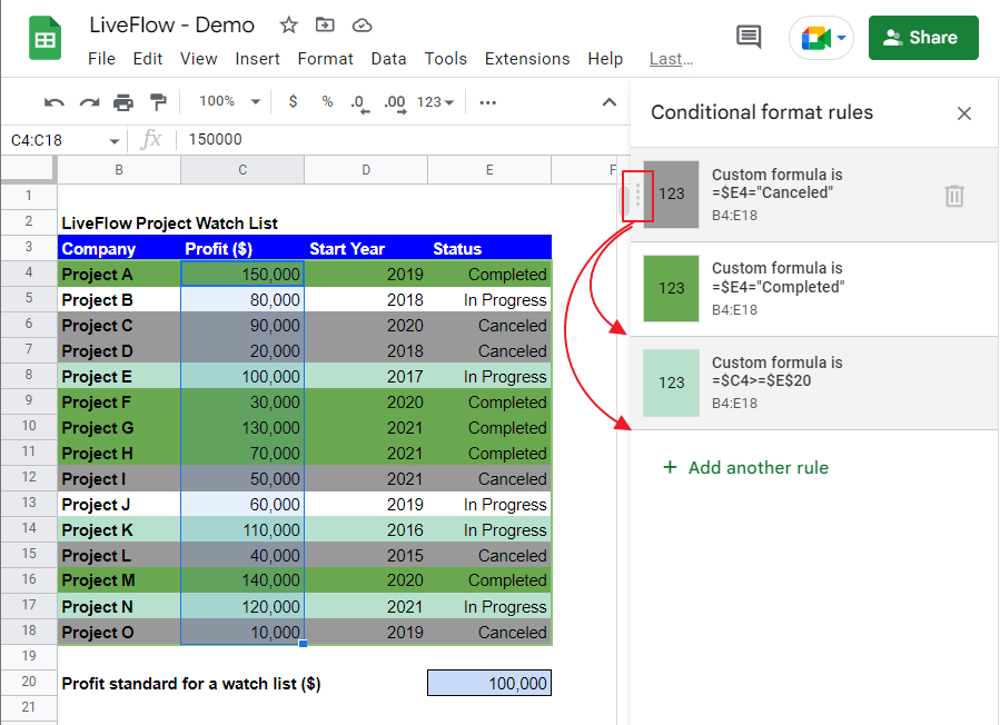
Google Sheets also offers a similar feature for applying conditional formatting based on another cell. Here's how you can do it:

1. Select the cell or range of cells you want to format based on another cell.
2. Go to the "Format" menu and select "Conditional formatting."
3. In the "Conditional formatting rules" sidebar, click on the "Add new rule" button.
4. Choose the desired rule type (e.g., "Color scale," "Text contains," "Custom formula is," etc.).
5. Depending on the rule type you selected, you'll need to specify the condition or criteria. For example, if you choose "Custom formula is," you can enter a formula that references the cell you want to base the formatting on.
6. Click on the "Formatting style" button to choose the desired formatting style (e.g., cell color, font style, etc.).
7. Click "Done" to apply the conditional formatting rule.

Example 2: Coloring Cells Based on Text in Another Cell (conditional formatting based on another cell)

Suppose you have a spreadsheet with student grades, and you want to color the cells in column C (Grade) based on the text in column B (Performance). Specifically, you want to color the cells green if the Performance is "Excellent," yellow if it's "Average," and red if it's "Poor."

Here are the steps:

1. Select the range of cells in column C that you want to format (e.g., C2:C100).
2. Go to "Format" > "Conditional formatting."
3. Click "Add new rule."
4. Select "Text contains" as the rule type.
5. In the "Text contains" field, enter "Excellent."
6. Click "Formatting style" and choose a green fill color.
7. Click "Done."
8. Repeat steps 3-7, but this time, enter "Average" and choose a yellow fill color, and then enter "Poor" and choose a red fill color.

Now, the cells in column C will be colored green if the corresponding cell in column B contains the text "Excellent," yellow if it contains "Average," and red if it contains "Poor."

Tips for Better Creating conditional formatting based on another cell in Google Sheets

While the examples above demonstrate the basic principles of conditional formatting based on another cell, there are many advanced techniques and scenarios you can explore. Here are a few additional tips and tricks:

• Use logical functions like AND, OR, and NOT to combine multiple conditions or criteria.
• Apply conditional formatting based on the value of multiple cells by referencing them in your formula.
• Utilize relative and absolute cell references to apply formatting rules across rows or columns dynamically.
• Explore other formatting options, such as icons, data bars, or custom number formats, to enhance the visual representation of your data.
• In Excel, you can create custom formatting rules using Visual Basic for Applications (VBA) code for more complex scenarios.

Conclusion

Conditional formatting based on another cell is a powerful technique that can greatly enhance the visual appeal and clarity of your spreadsheets. By highlighting or emphasizing specific data points based on the values or conditions of other cells, you can quickly identify patterns, outliers, and important information.

Whether you're working with sales data, student grades, or any other type of data, conditional formatting based on another cell can help you make more informed decisions and communicate your findings more effectively.

Remember to experiment with different formatting styles, conditions, and criteria to find the best way to visualize your data. And don't hesitate to explore advanced techniques and resources to further expand your conditional formatting skills.

Happy formatting!

Google Sheets AI Formula Generator | Formula Builder | Anakin.ai

Want to effortlessly create Google Sheets Formulas? This AI tool is here to help you easily create Google Sheets Formula Generator with ease!

Sam AltwomanSam Altwoman2

FAQ: Conditional Formatting Based on Another Cell

Can I conditionally format a cell based on another cell?

Yes, you can conditionally format a cell based on the value or condition of another cell in both Excel and Google Sheets. This technique allows you to apply formatting rules (such as cell color, font style, or icons) to a cell or range of cells based on the value or content of a different cell or range.

How do I color cells in Excel based on the value of another cell?

To color cells in Excel based on the value of another cell, follow these steps:

1. Select the cells you want to format.
2. Go to the "Home" tab and click "Conditional Formatting" > "New Rule."
3. Select "Use a formula to determine which cells to format."
4. In the formula box, enter a formula that references the cell you want to base the formatting on (e.g., =$A1="Done").
5. Click "Format" and choose the desired formatting style (e.g., green fill color).
6. Click "OK" to apply the rule.

Can I use an if formula in conditional formatting?

Yes, you can use an IF formula in conditional formatting to apply formatting based on multiple conditions or criteria. In Excel, when creating a new conditional formatting rule, select "Use a formula to determine which cells to format" and enter an IF formula that references the cells you want to base the formatting on.

How do I apply conditional formatting from one cell to another?

To apply conditional formatting from one cell to another in Excel or Google Sheets, follow these steps:

1. Select the cell or range of cells you want to format based on another cell.
2. Apply the desired conditional formatting rule, using a formula that references the other cell (e.g., =$A1>10).
3. If you want to apply the same formatting to other cells, copy the formatting by selecting the formatted cell(s), then click the "Format Painter" button.
4. Select the other cells you want to apply the formatting to.